FE 'tkGooie' Utilities

'ODEtools' group
of the
'MATHtools' group

Tool to Simulate
a Bouncing Ball

(No Air/Fluid Resistance)
(including an animation
on a Tk 'canvas')
(FE = Freedom Environment)

FE 'tkGooie' interface for
simulation of a bouncing ball.

Large, hi-res image is below.

FE Home Page >

FE Downloads Page or FE Overview Page >

FE 'tkGooies' Description Page >

FE 'tkGooies' 'MATHtools' Page >

FE 'tkGooies' 'ODEtools' Page >

This
'tkSimulateBouncingBall'
tkGooie Page

INTRODUCTION to Tcl-Tk script
'tkSimulateBouncingBall'

For at least 5 years now (about 2011 to 2016), I have had it on my Tk-scripts-to-do list to implement Tcl-Tk GUI scripts that perform numerical-integration of the ODE's ( ordinary differential equations ) that describe some dynamic physics configurations of classical mechanics --- as well as handling some non-physics applications.

I had in mind the 'ordinary'differential equations (ODE's) describing

  1. an oscillating pendulum,
    including wide-swinging,
    involving a non-linear ODE

  2. a bouncing ball

  3. a spring-mass-damper system,
    including non-linear

  4. projectile flight,
    including non-linear air resistance

  5. 2 gravitating bodies (in 2D),
    such as a planet and its moon --- OR
    a sun and its comet --- OR
    a planet and an orbiting satellite

  6. 3 gravitating bodies (2D and 3D)
    such as sun, planet, moon --- OR
    sun and two planets --- OR
    binary suns and a planet

  7. N gravitating bodies (2D and 3D),
    where N is greater than 3,
    such as a solar system

  8. predator-prey populations,
    such as wolves and moose --- OR
    moose and ticks --- OR
    wolves and moose and ticks

  9. populations subject to limits on growth,
    such as habitable area, cultivatable area, water resources, endless wars, epidemics

  10. pharmacokinetics
    (distribution of chemicals and their metabolites in the body of humans and other animals)

  11. chemical reaction kinetics

  12. etc.


A side note:

The first seven of the items above involve gravity.

Thanks to Isaac Newton (around 1700) and his successors, we know how to mathematically attack these types of problems.

Newton took a very Euclid-like geometric approach.

It took a couple of hundred years to develop the differential equations methods (and numerical integration techniques ) that are used today.

Runge and Kutta did their work around 1900.


Introduction (continued)

Recently (July 2016), I finally implemented a Tk script to simulate a single oscillating pendulum.

That 'tkGooie' script integrates the 'nonlinear' second-order differential equation that can be used to simulate the motion of a wide-swinging pendulum --- that is, there is no need to restrict the situation to small angular oscillations of the pendulum.

That Tk GUI script allowed for animating a representation of a pendulum arm-and-bob --- on a Tk 'canvas' widget.

I wanted to make a similar script that solves a second-order differential equation that can simulate a bouncing ball --- and provide an animation of the bouncing ball, using an image drawn on a Tk 'canvas' widget.

One reason that I wanted to do the bouncing ball simulation is because, many years ago (around 1970 to 1980), I gained experience in using the CSMP (Continuous System Modeling Program) software system that was available from IBM to run on IBM mainframe computers.

CSMP was a FORTRAN-like language that essentially extended the FORTRAN programming language to allow use of an 'INTGRL' function to perform the numerical integration process used to solve 'ordinary' differential equations.

I had devised a method of simulating a bouncing ball using CSMP.

That method involved a bit of 'trickery' with a 'NOSORT' option of CSMP to implement a 'velocity flipping at impact' technique.

I wanted to see how I could do that with Tcl-Tk.

    R.I.P. CSMP and DSL

    The same technique worked in DSL (Dynamic Simulation Language) which IBM eventually offered as a replacement for CSMP on their mainframe computers.

    CSMP and DSL 'died out' around 1995.

    Those software codes were no longer being supported by IBM.

    It is becoming almost impossible to find any guides or descriptions or examples of CSMP code on the internet.

    IBM seems to have done a good job of burying that bit of its past.

    But there may be some old descriptions available via amazon.com (used books).

    When you CAN find an old manual on the internet, it is usually a scanned PDF file that is slow to load and slow to page through.

    Here is a 24 page article from 1966, a relatively efficient PDF file, preserved at the Computer History Museum, that gives a description of DSL (PDF, 1.5 Megabytes, 24 pages).

    This can give an idea of what the CSMP and DSL languages were like.

    If you want to try loading and reading a 'scanned PDF' of a CSMP manual, here is a 1977 IBM CSMP User's Manual (PDF, 4.4 Megabytes, 77 pages) --- but be forewarned, it will be slow to 'turn the pages'.

    If you can find an IBM CSMP "Programmer's Guide", it may provide a better guide to the syntax and workings than the "User's Manual".

Introduction (continued, again)

To model the bounce, rather than using a 'stiff' differential equation, I used an algebraic method, integrated into the numerical integration process, to model the bounce --- by 'flipping' the velocity of the ball at the bounce.

This involved using an 'IF' statement in a CSMP 'NOSORT' section to set a velocity variable, V say, to minus V when the ball met (or went below) the surface on which it was bouncing.

I was curious how I could implement the same method ('velocity flipping') in a Tcl-Tk script --- along with an integration method such as Runge-Kutta 4th order (RK4) integration.

Since I had implemented an RK4 'proc' in the Tk script to simulate a single oscillating pendulum, a lot of the work was already done.

I 'just' needed to implement the 'velocity flipping' logic into that code --- along with some changes to the GUI.

I managed to implement the technique --- and that is the subject of this page --- with the code provided at a link below.


The Differential Equation to be Integrated

The form of the differential equation is the simple equation for a falling body near the surface of the Earth (or some other large, gravitationally attracting body --- such as the Earth's moon).

To simulate the falling ball means doing numerical integration of a simple, '2nd order' differential equation of the form


   D(D(u)) = -g

   where D represents the time-derivative operator d/dt,

     and t represents the time independent variable,

     and u represents the height of the center of the ball
           above the surface on which it bounces,

     and g is the acceleration due to gravity (on Earth or
           the Moon or Mars or a mountain-top or whatever).


This form of the ODE (ordinary differential equation) for a single, falling mass (the ball) assumes that there are no frictional forces (such as air resistance) during the flight. (More on this later.)

We assume that the ball is rigid and that when the ball hits the (also rigid) surface, the height u is the radius of the ball.

We let the height u be measured such that it increases in the upward direction --- with u = 0 being the height of the surface point on which the ball bounces.

Then the velocity D(u) of the falling mass is negative (downward).

    (You can convince yourself of this if you think of the velocity as being delta-height over delta-time, and observe that for the falling mass, delta-height is negative while delta-time is positive.)

Also note that because the velocity is getting 'more and more negative' as the mass falls, the acceleration is negative.

    (Delta-velocity over delta-time is a negative number over a positive.)

Since we let 'g' be a positive constant, we need the negative sign in front of 'g' in the expression above for the instantaneous acceleration of the mass at any time t.

---

Thank you, Galileo

Galileo showed that if one releases a mass and allows it to fall freely under the influence of an accelerative attraction toward the center of the earth, then the distance the mass falls in any time t from the time of release at rest (i.e. starting with zero velocity) is

g * t^2 / 2 --- g times t squared over 2.

Actually, the concept of a gravitational constant, g, came after his time.

Galileo showed that the distance fallen is proportional to the time squared.

And he noted that the rate of change of the velocity (the acceleration) seemed to be constant.

    But Galileo did not realize that gravitational acceleration declined as the square of the distance from the center of the Earth.

    It was Robert Hooke and Isaac Newton who came to that conclusion about 40 years after Galileo's death.

In any case, note that the mass of the ball is not involved in the expression relating distance to time.

This corresponds to the fact that Galileo observed that different masses, dropped from the same height, hit the ground at the same time.

    (He actually used spherical masses rolling down a linear inclined path, so that he could get fairly accurate measurements of the time elapsed in travelling to various distances along the inclined path.

    He adjusted the incline so that the ball rolled slow enough to get the time measurements.)


It was a beautiful piece of furniture that Galileo
used in his gravitational acceleration experiments.
They don't make 'em like that anymore. (Note the hardware
that tripped little bells when the sphere/mass rolled through.)

Reference: Museo Galileo

So, from what Galileo discovered, we learned that we do not need numerical integration to solve the simple ODE

D(D(u) = -g.

If the initial height at time zero is denoted u(0), and the ball is dropped (initial velocity is zero), the height at time t is given by

u(0) - g * t^2 / 2

However, in spite of the fact that we have a simple algebraic expression for the solution of the ODE, we use numerical integration to do the solve.

This makes it relatively easy to handle additional terms describing effects like air resistance --- which is related to the downward or upward velocity of the ball.

    Note that if the ball is still, there are no forces on it.

    The ball has to be moving for air resistance force to be generated.

    Hence a mathematical expression for the air resistance will involve numbers for motion of the ball, such as velocity, and the height of the ball plays no part in the expression for deceleration due to air resistance (if the range of heights is relatively small).

    (Of course, height can play a part --- for example, when we are dealing with different air density at different heights --- or different wind currents at different heights.)

If air resistance is proportional to the magnitude of the velocity or to the velocity squared or some combination of the two, then we can use numerical integration to solve a differential equation that may look something like

D(D(u)) = -g -k1*D(u) -k2*sign(D(u))*D(u)^2

where D(u) represents the signed velocity of the ball.

    Although this equation still does not explicitly involve the mass of the ball, note that the constants of resistance, k1 and k2, will surely depend on factors like the profile of the ball, like its radius, and the density of the air.

    In some situations, mass of the falling object WILL come into play.

    If we were simulating a feather-weight falling object, we would find that the density of the air versus the density of the falling object would have a definite effect on the deceleration of the object.

    Think of a falling ping-pong ball versus a golf ball.

For now, I aim to simulate the no-air-resistance case.


MODELLING THE BOUNCE

(in an algebraic way, rather than using
an extremely 'stiff' differential equation
to model what happens during a nearly
instantaneous bounce)

We model the bounce by switching the velocity direction of the ball when it strikes the surface --- when height u is less than or equal to the radius of the rigid ball --- so the velocity D(u) is set to -D(u).

To allow for modeling a ball that is losing height with each bounce because of a loss of some momentum with each impact with the surface, we introduce a positive constant k which is less than or equal to 1.

When we switch the direction of the velocity, we also reduce the velocity magnitude by the factor k.

Hence the velocity D(u) becomes -k*D(u) at each bounce.
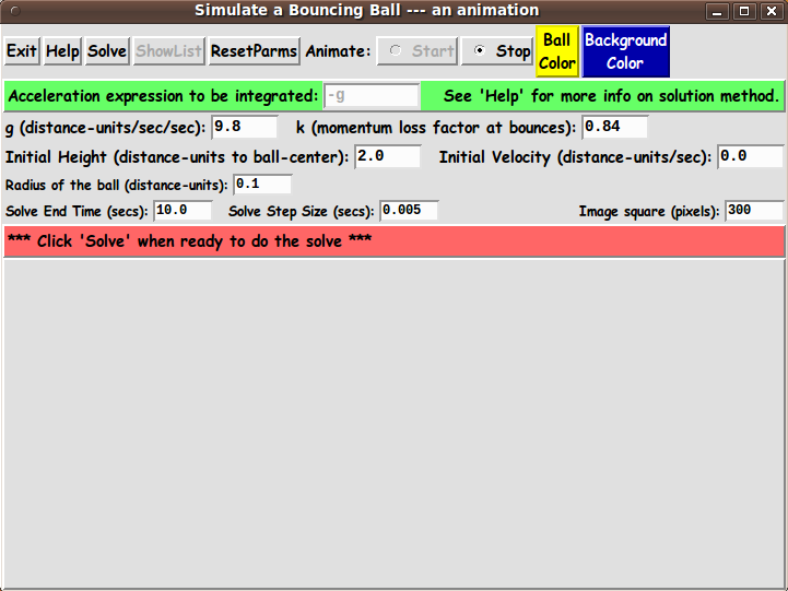

GOALS FOR THE GUI:

The GUI should allow the user to enter various values for g (gravity) and k (velocity adjustment at each bounce).

    (Note that the differential equation D(D(u)) = -g does not involve mass --- as mentioned above.

    So we do not have to prompt for mass on the GUI.)

To be able to do the numerical integration of the 2nd order ODE, we need a couple of initial conditions for the displacement u and the velocity D(u).

The GUI should allow the user to enter four parameters for the solver process:

  • an initial vertical height of the ball

  • an initial vertical velocity
    (zero for a ball that is dropped rather than thrown)

  • an end-time for the end of the solution process

  • a time-step, h, for the solution process.

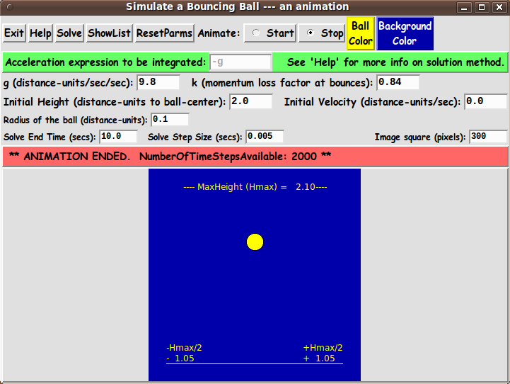
Following a solution run, the GUI should also allow the user to start (and stop) an animation of the bouncing ball drawn on a Tk canvas.

The moving ball is to be shown on a square Tk 'canvas' widget, centered in a rectangular image-area --- by using 'create oval' and 'delete' commands on the Tk 'canvas' widget.

---

To evaluate any further requirements that we may need for the GUI, it is helpful to know some of the details of

  • the method of numerical integration of the differential equation

  • the method of implementing the animation

Those details follow.


METHOD - MATH MODELLING OF THE BOUNCING BALL MOTION :

To make the problem compatible with numerical integration methods, we convert the single 'second order' differential equation

D(D(u)) = -g

to two differential equations with u1 = u = displacement and u2 = D(u) = velocity as the functions of t to be generated by integrating 2 'first order' differential eqns:

      D(u1) = u2
      D(u2) = -g

starting from initial conditions u1=A and u2=B, where A is an initial vertical height and B is an initial vertical velocity.

The common way of expressing these kinds of systems of first order differential equations in compact, general form is

D(u) = f(t,u)

where u and f are N-dimensional vectors.

This is a compact way of expressing a system of scalar differential equations:

D(u1) = f1(t,u1,...,uN)
D(u2) = f2(t,u1,...,uN)
. . . . . . . . . . .
D(uN) = fN(t,u1,...,uN)

In the case of these bouncing ball equations, N=2, and we can think of solving for the unknown function vector (u1(t),u2(t)) where the right-hand-side (RHS) of the two equations above can be thought of as a special case of a more general user-specified function vector

(f1(t,u1,u2),f2(t,u1,u2))

where

f1(t,u1,u2) = u2
f2(t,u1,u2) = -g

We use the popular Runge-Kutta 4th order method (RK4) to perform the numerical integration for a user-specified time step, h.

We basically use two procs to perform the integration steps:

  • a proc to perform the RK4 integration for N=2.

    This proc yields the values of (u1,u2) for each time step.

  • a proc to evaluate the RHS function (f1,f2) for specified values of t,u1,u2.

The latter proc ('deriv', say) is called several times by the former proc ('rk4', say) for each time step.


METHOD - PLOTTING THE ANIMATION ON THE TK CANVAS :

After a solution, we have the solution functions u1 and u2 for a sequence of (equally-spaced) time values.

    We could use a more complex Runge-Kutta method --- such as Runge-Kutta-Fehlberg --- to get a solution with potentially unequally-spaced time values.

We use function u1 (height of the ball) to do the animation.

For each time value, t(i), the bouncing ball is drawn as a simple color-filled circle representing the ball.

The GUI provides 2 buttons by which the user can specify the 2 colors for:

  • the canvas background

  • the bouncing ball (the circle) and a line representing the surface on which the ball bounces.

An 'animate' proc performs the bouncing ball animation when the user clicks on the 'Start' radiobutton of the GUI.

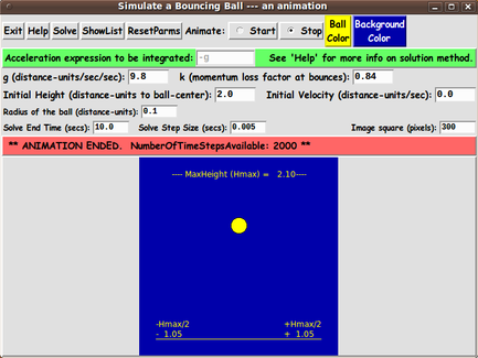
This 'animate' proc uses the 'world-coordinates' --- the values of height u1 --- to draw the bouncing ball within a square area of about Hmax-by-Hmax in world coordinates, where Hmax is the maximum height, over the surface on which the ball bounces, reached by the ball during a solve run.

We use u1 to represent the location of the center of the ball, so we need to adust the max height of the bounce by the radius of the ball to accomodate the top half of the ball.

We think of Hmax, below, as representing that 'augmented' height.

We think of the ball bouncing up and down in the y-direction, with no 'side' forces on the ball in the x-direction.

Hence the x-coordinate of the location of the ball stays constant.

We imagine the Hmax-by-Hmax square to have an xy-coordinate system overlaid on it such that the origin (0.0,0.0) is at the middle of the bottom of the square.

In other words, the y-coordinate of the square goes from 0.0 at the bottom of the square to Hmax at the top of the square --- and the x-coordinate goes from -Hmax/2 at the left side of the square to +Hmax/2 at right side of the square.

We think of the bottom of the path of the center of the rigid, extremely hard bouncing ball (non-squishable, like a golf ball) as being above the origin --- (0.0,ball-radius).

We use the height function u1(t(i)) of the center of the ball to set the y coordinate of the location of the center of the bouncing ball, and we keep the x-coordinate of the (x,y) position of the center of the ball at 0.0 --- the x-mid-point of the square.

Note that the x,y coordinates of the upper-left corner of the square are (-Hmax/2,+Hmax) and the lower-right corner of the square is at (+Hmax/2, 0.0).

The Hmax-by-Hmax area allows for the bouncing ball to bounce to extremes --- from height zero to height Hmax.

A proc is provided which maps the plot area limits in world coordinates --- say

      UpperLeftCorner: (-Hmax/2 , +Hmax)
      LowerRightCorner: (+Hmax/2 , 0.0)

to the corners of the plot area in pixel coordinates:

      UpperLeftCorner: (0 , 0)
      LowerRightCorner: (ImageWidthPx , ImageHeightPx)

We use values a little larger than Hmax and a little smaller than 0.0 for the world coordinate height limits --- to allow for a little margin at the top and bottom of the path of the bouncing ball.

To get a square image area, we use ImageWidthPx=ImageHeightPx and we determine this number of pixels by allowing the user to specify the integer value in an entry widget on the GUI.

The animate proc uses 2 procs --- Xwc2px and Ywc2px --- to convert the world coordinates of each point --- such as the location of the center of the bouncing ball --- to pixel coordinates.

The pixel-coordinates are used in the 'create oval' command to redraw the bouncing ball on the Tk canvas, for each time step.


THE GUI LAYOUT :

From the discussion above, we see that the Tk GUI should allow the user to specify

  • g   (gravitational acceleration at Earth's surface)

  • k   (a loss factor)

  • initial-height

  • initial-velocity

  • time-step-size

  • end-time

  • ball radius

  • and image size.

There is to be a 'Solve' button to perform a solution when the user is ready to use these parameters.

A 'ShowList' button can be used to show the list of solution values --- triplets t(i), u1(t(i)), u2(t(i)) --- in a popup window.

There are also to be 2 buttons by which to call up an RGB-color-selector GUI by which to specify the 2 colors for the animation drawing on the canvas.

In addition, on the GUI, there are to be 'Start' and 'Stop' radiobuttons to start and stop an animation run.

To allow the user to speed-up or slow-down the animation, there could be a Tk widget ('entry' or 'scale') by which to specify a wait-time (in millisecs) between computing and displaying each new bouncing ball position.

This would be an alternative to using a wait-time value calculated from the user-selected time-step, h.

For now, we simply calculate the animation wait-time based on the time-step, h.

---

One way the user can specify all these parameters is indicated by the following 'sketch' of a layout for the GUI:

In the following sketch of the GUI:


   SQUARE BRACKETS indicate a comment (not to be placed on the GUI).
   BRACES          indicate a Tk 'button' widget.
   UNDERSCORES     indicate a Tk 'entry' widget.
   A COLON         indicates that the text before the colon is on a 'label' widget.
   CAPITAL-O       indicates a Tk 'radiobutton' widget.
   CAPITAL-X       indicates a Tk 'checkbutton' widget (if any).
   Vertical bars (and horizontal hyphens) outline a 'canvas' widget.
   
   If there are scrollbars:
   Less-than and greater-than signs indicate the left and right ends of a horizontal 'scrollbar'.
   Capital-V and Capital-A letters indicate the bottom and top ends of a vertical 'scrollbar'.


Here is the sketch :

FRAMEnames
VVVVVVVVVV
            ------------------------------------------------------------------------------------------
            Simulate a Bouncing Ball --- an animation
            [window title]
            ------------------------------------------------------------------------------------------

.fRbuttons   {Exit} {Help} {Solve} {Show {Reset  Animate: O Start O Stop  {Ball   {Background
                                    List} Parms}                           Color}     Color}

.fRrhs       [ ....  A description of the equation(s) or solution technique goes here, in a label widget.  ....... ]
             [This could be an entry widget, someday, to allow for changes in the math expression for acceleration.]

.fRfactors   g (distance-units/sec/sec): 9.8__   k (momentum loss factor at bounces): 0.95_

.fRinit      Initial Height (distance-units of ball-center): 2.0___  Initial Velocity (distance-units/sec): 0.0___

.fRball      Radius of the ball (distance-units): 0.1___

.fRtime      Solve End Time (secs): 10__   Solve Step Size (secs): 0.05___          Image square (pixels): 300__

.fRmsg       [ ..........  Messages go here, in a label widget .......................... ]

.fRcanvas    |------------------------------------------------------------------------|
             |                                                                        |
             |     [This area is to contain a non-scrollable square canvas widget     |
             |      in which the animation is to be drawn.                            |
             |                                                                        |
             |      The square canvas widget is centered at the top of this area.]    |
             |                                                                        |
             |                                                                        |
             |                                                                        |
             |                                                                        |
             |------------------------------------------------------------------------|


GUI components:

From the GUI 'sketch' above, it is seen that this GUI layout consists of about

  • 7 button widgets
  • 11 label widgets
  • 8 entry widgets
  • 1 canvas widget with no scrollbars
  • 2 radiobutton widgets in 1 group
  • 0 scale widgets
    (but may use scale widgets in place of some entry widgets)
  • 0 checkbutton widgets
  • 0 listbox widgets
  • 0 text widgets

The GUI (a screenshot)

To implement this Tk GUI script, I fetched the

'tkSimulatePendulumNoFriction' script

that had most of these GUI elements and converted it to a 'tkSimulateBouncingBall' script.

I ended up with the GUI seen in the following image.

This is the GUI as it first appears.

As the message in the middle of the GUI indicates, the user can take the defaults for all the parameters and simply click on the 'Solve' button to do the numerical integration.

Just as I found with the

'tkSimulatePendulumNoFriction' script,

when I run the solve-process with this set of values, it is astonishing how quickly the solve completes --- in a fraction of a second!

A 'solve completed' message appears in the message area so quickly after you click on the 'Solve' button that, if you blink, you may not notice any change in the GUI and you may not realize that the solve is already done.

The 'SOLVE DONE' message said that the elapsed time for the solve was 279 milliseconds --- less than one-third of a second for 2,000 time-steps of integration.

Not bad, considering I have not expended time trying to obtain the optimum speed out of all the numerical integration code.

When I clicked on the 'ShowList' button, a list of the computed results --- time, height (in distance-units), and velocity (in distance-units per second) --- appeared for the 2,000 time steps and corresponded to the default initial conditions.

---

Note that you can use the 'ShowList' button to generate columns of decimal numbers that can be copied-and-pasted into a text-editor window.

The text editor can be used to save the data to a text file.

Then that text file can be edited (to remove or comment out the header and trailer text) and the file fed into a 'tkGooie' plot utility such as

tkGnuplotXY_2or3colsFromFile

to get a plot of the height and/or velocity functions versus time.

---

To give you an idea of what the animation image area looks like, below is a 'screenshot'.

Before clicking the 'Start' button for this animation, I could have used the 2 color buttons to call up a color selector GUI to set the ball color to white and the background color to black, for example.

---

HELP TEXT

The 'Help' button on the GUI shows extensive text describing this utility, in a popup window with scrollbars for the text area.


DESCRIPTION OF THE CODE

Below I provide a link to the Tk script code for this 'tkSimulateBouncingBall' utility.

For this Tk script, I follow my usual 'canonical' structure for Tk code:


  0) Set general window & widget parms (win-name, win-position,
     win-color-scheme, fonts, widget-geometry-parms, win-size-control,
     text-array-for-labels-etc).

  1a) Define ALL frames (and sub-frames, if any).
  1b) Pack   ALL frames and sub-frames.

  2) Define & pack all widgets in the frames, frame by frame.
     Within each frame, define ALL the widgets. Then pack the widgets.

  3) Define keyboard and mouse/touchpad/touch-sensitive-screen action
     BINDINGS, if needed.

  4) Define PROCS, if needed.

  5) Additional GUI initialization (typically with one or more of
     the procs), if needed.


This Tk coding structure is discussed in more detail on the page A Canonical Structure for Tk Code --- and variations.

This structure makes it easy for me to find code sections --- while generating and testing a Tk script --- and when looking for code snippets to include in other scripts (code re-use).

I call your attention to step-zero.

One thing that I started doing in 2013 is using a text-array variable --- named 'aRtext' --- for text in labels, buttons, and other widgets in the GUI.

This can make it easier for people to internationalize my scripts.

I will be using a text-array like this in most of my scripts in the future.


Experimenting with the GUI

As in all my scripts that use the 'pack' geometry manager (which is all of my 100-plus scripts, so far), I provide the four main 'pack' parameters

  • '-side'
  • '-anchor'
  • '-fill'
  • '-expand'

on all of the 'pack' commands for the frames and widgets.

That helps me when I am initially testing the behavior of a GUI (the various widgets within it) as I resize the main window.

I think that I have used a nice choice of the 'pack' parameters.

In particular ...

The labels and buttons and entry widgets stay fixed in size and relative-location as the window is re-sized --- while the area containing the 'canvas' can expand/contract as the window is re-sized.

You can experiment with the '-side', '-anchor', '-fill', and '-expand' parameters on the 'pack' commands for the various frames and widgets --- to get the widget behavior that you want.

---

Additional experimentation with the GUI:

You might want to change the fonts used for the various GUI widgets.

For example, you could change '-weight' from 'bold' to 'normal' --- or '-slant' from 'roman' to 'italic'.

Or change font families.

In fact, you may NEED to change the font families, because the families I used may not be available on your computer --- and the default font that the 'wish' interpreter chooses may not be very pleasing.

I use variables to set geometry parameters of widgets --- parameters such as border-widths and padding.

And I have included the '-relief' parameter on the definitions of frames and widgets.

Feel free to experiment with those 'appearance' parameters as well.

---

Note that the color buttons call on a color-selector-GUI script to set the colors.

You can make that color-selector script by copying-and-pasting the code from the page offering 'a non-obfuscated color selector GUI', on this site.

Some comments and code at the bottom of this 'bouncing ball' Tk script explain how you can implement the RGB color selector script.


Some features in the code

There are plenty of comments in the code, to describe what most of the code-sections are doing.

You can look at the top of the PROCS section of the code to see a list of the procs used in this script, along with brief descriptions of how they are called and what they do.

---

Below is a brief overview of the procs of the script.


  - 'solve'                    - called by the 'Solve' button.

                                (The 'velocity flipping' logic needs to be in this proc,
                                 not in the 'runge-kutta-4' proc called by this proc.)

  - 'runge-kutta-4'            - called by the 'solve' proc.

  - 'deriv'                    - called by the 'runge-kutta-4' proc.

  - 'show_list'                - called by the 'ShowList' button

  - 'animate'                  - called by a click on the 'Start' animation radiobutton.

  - 'setMappingVars_for_px2wc' - called by proc 'animate'.

  - 'Xwc2px'                   - called by proc 'animate'.
  - 'Ywc2px'                   - called by proc 'animate'.

  - 'set_ball_color1'          - called by the 'BallColor' button.

  - 'set_background_color2'    - called by the 'BackgroundColor' button.

  - 'update_color_button'      - sets background & foreground color of
                                 either of the 2 color buttons.

  - 'advise_user'              - called by the 'solve' and 'animate' procs.

  - 'reset_parms'              - called by the 'ResetParms' button and in the
                                 'Additional GUI Initialization' section,
                                 to initialize the parms.

  - 'edit_inputs'              - called by 'solve' and 'animate' procs

  - 'decimal_check'            - called by 'edit_inputs' proc

  - 'popup_msgVarWithScroll'   - called by the 'Help' button.


The main numerical integration code is in the 'runge-kutta-4' and 'deriv' procs.

See the comments in those procs for details on their implementation.


A fervent hope

It is my hope that the copious comments in the code will help Tcl-Tk coding 'newbies' get started in making GUI's like this.

Without the comments, potential young Tcler's might be tempted to return to their iPhones and iPads and iPods --- to find videos of Donald Trump or news articles about him, when gasoline prices in the U.S. were exceeding 4 dollars per gallon and headed toward 5 dollars per gallon (around 2012) --- when he said that the U.S. should invade Canada and take their oil.

Hey, Canada. You had better build a wall.
Trump wants your oil.

Trump thinks it's OK to invade and conquer you, Canada.

If gasoline prices shoot up after he is elected, you can expect Trump to have the generals plan an invasion.

Before that happens (and civilization breaks down completely), Tclers, try installing-running-enhancing the following code.

To help out in making Tk scripts like this, here is

a page that provides sources of Tcl-Tk code snippets

by providing links to various 'tkGooies' scripts that can make it relatively quick work to compose

  • widget definitions,
  • bind statements, and
  • procedure code.

And when you get to the testing-and-debugging phase in development of a Tk script, here is

a page that describes the wonderfulness of the 'wish' 'stack trace' facility,

which can make the testing-and-debugging go relatively quickly and painlessly.

    By the way ... Canada ... if you build that wall

    make Trump pay for it.


The Tcl-Tk CODE :

Here is a link to CODE for the script

'tkSimulateBouncingBall.tk'.

With your web browser, you can 'right-click' on this link --- and in the menu that pops up, select an item like

'Save Link Target As ...'

--- to save this file to your local computer.

Then you can rename the file to remove the '.txt' suffix.

Make sure that you have execute permission set on the file --- in order to execute the script.


SOME POTENTIAL ENHANCEMENTS:

Some features that I may add to this Tk script --- or implement in a separate Tk script:

  • ALLOW FOR SPECIFYING THE RHS MATH EXPRESSION, instead of parameters:

    This GUI could be used for a wide variety of 'tweaks' to the math expression for the RHS (right-hand-side) of the DE for acceleration.

    This could be accomplished by 'activating' the 'entry' widget on the 'green' text line of the GUI --- the line that currently simply shows the RHS --- '-g' --- of the second-order DE that is to be solved.

    That 'entry' field could hold a mathematical expression.

    For example, a term to account for air resistance could be introduced --- along with '-g'.

    The 'deriv' proc would need to be updated to handle an expression that could be placed in the entry widget.

    The initial expression could be one like the one for air resistance discussed above:

    -g -k1*D(u) -k2*sign(D(u))*D(u)^2

    in a form like

    -g -k1*$v -k2*sign($v)*$v^2

    where g, k1, and k2 could be 'hard-coded' constants that the user could change,

    and where $v is a variable being used internally by the 'deriv' proc to represent the velocity variable.

  • PROVIDE A PLOT OPTION,
    to do a plot of u=u1 and D(u)=u2
    versus time
    :

    We could add a 'Plot u,D(u)' button to the top of the GUI to enable using the canvas area of the GUI to do an 'xy' plot --- as well as using the area to do animations of the bouncing ball.

    A new 'plot' proc (and associated procs) would need to be added.

    This would add a lot of code to this already-long Tk script.

    It is probably better to simply provide the 'ShowList' option and let the user transfer that output to a plot utility --- UNLESS you want to make plotting from this utility as simple as a 'click on a button'.

  • PROVIDE A MORE ACCURATE HANDLING
    OF THE 'VELOCITY FLIPPING' at impact
    :

    In general, in the integration step when the ball hits the surface, the height of the center of the ball goes (mathematically) slightly below the radius of the ball.

    In this first release of this script, I reset the height of the ball to its radius and I flip the velocity.

    However, the velocity that is flipped is slightly larger (in the negative direction) than it should be, for almost every bounce.

    I should correct the velocity before flipping it.

    Currently the result is that the ball is rebounding slightly faster (and higher) than it should.

    One can eliminate most of this error by simply using a smaller integration step-size, h --- as a rough work-around.

    I have in mind a way to correct the velocity for the 'over-shoot', before 'flipping' the velocity.

    The technique takes quite a few paragraphs to describe clearly.

    Here is a quick summary of the several steps.

    • Let du1 = ( u1(t+h) - radius-of-ball ) denote the 'height overshoot' of the ball --- more like an 'undershoot' since it is negative.

    • Let dt denote the 'time overshoot'.

      Gallileo et. al. gave us the relationship of delta-displacement in terms of delta-time:

      du1 = -g * (dt)^2 / 2

      We rearrange that expression to give dt in terms of du1.

    • We then can calculate the 'velocity overshoot' dv = -g * dt.

    • Finally, we use the 'velocity overshoot' ( dv ) and the 'time overshoot' ( dt ) to correct the velocity, u2, and the time, of the bounce --- as well as correcting the 'height overshoot' by setting the height u1 to be the radius of the ball.

    • We essentially re-start the simulation --- from the corrected time-point (which is now not necessarily a multiple of h) --- continuing to take time-steps h.

    I may update this script in the future with this better way of handling the 'velocity flipping' at each bounce --- probably if/when I implement the following enhancement --- an option to easily create an animated GIF file.

  • PROVIDE AN OPTION to
    SAVE AN ANIMATION
    as an ANIMATED GIF File
    (or as a movie file, such as a '.mp4' file).

    A 'WriteAniGIF' (or 'WriteMovie') button could be added to the GUI, and a technique like that used in the

    of the FE 'tkGooies' system could be used to make an animated GIF file.

    This enhancement would (like a plot option) add a lot of code to this already-long Tk script --- but it might be worth it --- to make capturing an animation as easy as 'falling off a log'.

---

There will probably be more enhancements that I may think of in the future, although some enhancements might be more worth the effort of implementing if put in a different Tk script --- like a 'solar system' script

--- perhaps using somewhat different equations (for example, no 'velocity flipping') or different GUI design (including a 'WriteAniGIF' option?) or different numerical methods (perhaps a Runge-Kutta-Fehlberg method).


IN CONCLUSION

There's a lot to like about a utility that is 'free freedom' --- that is, no-cost and open-source so that you can modify/enhance/fix it without having to wait for someone else to do it for you (which may be never).

I hope to provide more free scripts that can be used to demonstrate mathematical principles (and Tk coding techniques) --- scripts that could be used in a classroom or self-teaching setting.

As I have said on other 'tkGooie' pages of this FE web site ...

A BIG THANK YOU to Ousterhout for starting Tcl-Tk, and a BIG THANK YOU to the Tcl-Tk developers and maintainers who have kept the simply MAH-velous 'wish' interpreter going.

Bottom of this page for
presenting Tcl-Tk code for GUI
tkSimulateBouncingBall
--- a utility in the FE 'tkGooies' system,
in the 'ODEtools' subgroup
of the 'MATHtools' group.

To return to a previously visited web page location, click on the Back button of your web browser a sufficient number of times. OR, use the History-list option of your web browser.
OR ...

< Go to Top of Page, above. >

Page history:

This FE web page was created 2016 Jul 17.

This FE web page was changed 2016 Jul 23.
(Added to the 'Potential Enhancements' section --- and corrected some typos.)

This FE web page was changed 2016 Jul 30.
(Added links to 2 programming aid pages and an abbreviated description of enhanced 'velocity flipping' logic for the bounces.)

Page was changed 2019 Mar 04.
(Added css and javascript to try to handle text-size for smartphones, esp. in portrait orientation.)

Page was changed 2019 Jun 28.
(Specified image widths in percents to size the images according to width of the browser window.)


NOTE:
This code and description has not been posted on a Tcler's Wiki page --- at wiki.tcl-lang.org --- formerly wiki.tcl.tk. If I ever do so, as a backup and alternative to this page, I plan to add a link to that Wiki page here.